


Abstract
Many software packages are available for power systems network simulation, some of which are freely available. GridLAB-D Is a popular open source choice for smart grid research and allows users to have complete control over the production of the network via C++ style object based programming of the model file. A lack of GUI restricts the use of the software to small hand written systems but lends itself to script based creation of large network models. To allow new users an easy way to learn how data is structured in GLD without having to immediately learn the language and to provide better tools for conversion into GLD models, a standard data format is created. This standard can be used to manually format data and have model data automatically converted to. Data in this form can then be converted into a GLD model using a MATLAB script.
Development of a Standard Form for Conversion to GridLab-D
A large network will be used to conduct experiments and must therefore be converted into GLM format. Adjustments can be made to the system at will to conduct many experiments in computer simulation, testing for optimal transactive solutions on the campus. Both small and large campus networks are based on a real network. Coincidence between the Power*Tools and GridLab-D simulations gives confidence that transactive experiments will have reasonable accuracy to the real system on campus.
A small 72 node network is a portion of the large campus wide 2612 node network. This small network is a substation of the large network and was ported as described below. It was used to verify the standard and the conversion script, but it was also used to verify the coincidence of results to PTW to confirm the usefulness of the model and GLD as tools for transactive experiments. Results agreeing between the two software packages indicates the construction of the model is correct. Experiments can therefore be done with confidence that they pertain to the actual function of the physical system.
Since the large network is the network of interest it is the most important to ensure that it is modeled properly. It and the small system were converted to GLM format as follows.
General Overview of the Standard
Information essentially links across files in the Standard, referencing components, nodes, and configurations. It is made clear by the formatting of the file that all visible information constructs the listed objects, yet references can be made to other files to append data or indicate physical connections of components. Configurations are made apparent and the files for those configurations can be understood at a glance. All parameters are referenced in the same place in the files at all times.
The format of connections in GLD is based on a from-to system, though other systems are easily transferable. Power*Tools formats connections as direct to other components rather than via nodes. A differing paradigm such as this is not an issue for a standard format since the conversion from the standard could easily recognize it and accommodate.
As it stands, there are 19 Standard Files being used, all of which are based on a common form with requisite attributes added where necessary. Nodes and lines in GLD both require a unique designator/name, phase information, and voltage information, but they do not both have lengths and connections; these are only required for the cable Standard File. This is the case for all Standard Files, ensuring similar information is in the same place, but different component types have designated files in which they will reside for later checking and easy retrieval during conversion. This data can be entered or omitted where necessary whist it being obvious when either is done.
Configurations make duplicating content simple. Just as configurations in GLD and libraries in other software, the Standard Form configurations act as a list of different forms of a certain objects type. These specialized forms can be used in lieu of populating the same data across many different objects. If two lines should be constructed in the same manner, but with different lengths, then the length can be defined for each in the line file while each can be given the same configuration. The configuration is used instead of the information that would otherwise construct the line, but across all lines which are designated with that configuration. A library of commonly use lines, transformers, or other objects can be made to allow easy manual population of the other files. Both automated file population and file population via conversion to the Standard Form can make use of these configurations. A stored library in the Standard configuration form can be used for many different file conversions, or a library can be converted into this Standard configuration form.
Conversion Method
PTW-to-Standard
The real campus models must be converted to GLD for verification of the standard and for their use in transactive power flow experiments. PTW models are used to verify the automated conversion to the Standard format. Small and large PTW models were sequentially converted to progressively improve the functionality of the standard and the conversion to GLD. These processes were done in conjunction with the development of the Standard-to-GLD conversion script and the Standard Files.
First a small model of 72 nodes is used to test. It is purely radial and only contains a few types of components; lines, loads, transformers, breakers, and fuses. The export from PTW is transformed to be more easily readable. MATLAB script created by Emily Fabian was used to convert the CSV export into a multi-tabbed XLSX. The purpose of this is to improve readability of the Export file.
As it comes from PTW, the exported CSV contains all data used to model the network. As can be seen in the PTW Exported Master Sheet Example below, different types of components are grouped together and select parameters for each group are given. Buses are considered one group, and parameters such as the name, nominal voltage, and short circuit rating are provided. Many parameters may not be of any use. Parameters may not have any information associated with them, may have sparse information, or contain information yet irrelevant. Other sections like ‘Cables’ contain information which describes the construction of all lines in the network. Much information here is unused to convert to the Standard Form. Some information refers to the libraries used in PTW but these databases are not available for export. Further sections such as 2-winding transformers, 3-winding transformers, utilities, and protective devices - containing breakers, fuses, relays, and reclosers - as well as separate load sections like, non-motor loads, induction motors and synchronous motors and many more are all represented in the export. Fabian’s code recognizes each new section and creates a new XLSX tabulated file with each section and property accounted for. Each section has a name which is used to designate it in the XLSX. When the Cable section is created the preface ’Ca_’ will be used to name all of the tabs in that sections; ‘Pr_’ for the protective devices, and so on. Each property in the section is analyzed for content. If the property is completely empty then it is excluded from the XLSX. If content is found in any single cell then the property is written to a new tab. For example, cable nominal voltages will be stored in the tab labeled ‘Ca_SystemNominalVoltage’. Each new section is written in this fashion, though it should be noted that careful attention should be paid to the naming of the sections in the master export file. If two sections have the same two initial letters then they will overlap and cause issues in the data. Overwriting, mixed data between sections, and missing properties can all occur due to non-unique section initials. Some manual work is required for the larger system since this will occur otherwise.
Once the XLSX is produced it can be used to easily put the model data into Standard Form. Another MATLAB script is used to read the requisite data from the XLSX. Only some properties are required to fill out the Standard Form, so only those are read. Just as the manual input of data is done, automatic input fills out the data in each file after creation. Configurations for PTW are not transferable from the databases in that software, thus no configurations are available, and every component must be written individually.
Being automated, this process does not take long. Although the Standard Files will become lengthy they will not become longer without these configurations, only more populated due to individual data entry instead of the configurations. Each required property is sought in the XLSX and if found is used to populate the current Standard File being produced. The script is built to specifically search each required property in each section. If a property is not found then that property in the Standard File is left unpopulated. The same is true for the files themselves. If there are no capacitors then no capacitor Standard File is created.
Some transformations are required since Standard Format uses different information than is provided in PTW export. Power should be in kW rather than MW so a multiplier of 1000 is applied, while electric potential should be in kV rather than V requiring a factor of 0.001.
Other adjustments must also be made to refine the data being input to Standard Form. Specifically the unique names of objects and the connections must be changed, though there is also encoded data which must be dealt with.
Names directly from PTW may contain any character though some of these may cause issues in GLD. Certain characters such as whitespace ( ), colon (:), ampersand (&), and comma (,) can cause issue in GLD and in MATLAB due to scripting use causing unwanted effects in the file, or offsetting comma separated values (CSV files).
The form of connections in PTW is also different from the common node-member/to-from based connections. Connections in PTW refer to other connections on other components. A connection called ‘fuse1:1’ would designate this connection to the first connection of the object called ‘fuse1’. A renaming algorithm was therefore created handle this.
The PTW naming scheme has directionality of objects, so this must be maintained in the transformation to a node-member system. A set of series objects would typically have connections as 1->2, 1->2,….,1->2; that is every second connection of a component would be connected to the first connection of another. Connections can also be made to the same numbered connection of another component. An added complication is the inclusion of buses. These act as nodes in PTW but are usually reserved for connections between 3 or more components. In the case of connection to a bus, the connection is always connected to the first connection ‘:1’ since the bus only has one connection point. Each of these types of connections must properly transform to reference a common node where connections are made. If ‘cable1” is connected to ‘fuse1’ their connections might look as follows: cable1 connection to ‘fuse1:1’, fuse1 connection to ‘cable1:2’. If the first connection of every component is renamed to be self-referential then the connection to it would be of the same name. In this example the fuse1 would change its first connection name from ‘cable1:2’ to ‘fuse1:1’. Since the second connection of cable1 is to ‘fuse1:1’ the two connections have now been transformed into node references, each calling on a common node and preserving the connection between the two components.
If connections are made to a common bus they will all reference the first connection of the bus, i.e. ‘:1’. The renaming scheme does not work here since all connections already properly reference a common node; the first connection of the bus. For example, if XFMR1 and relay1 are connected to bus2 then the connections would both be ‘bus2:1’ and no renaming should take place. To handle this, a check is made to see if the connection is to ‘:2’. If the connection is made to a second connection of another component then the self-reference scheme is used, otherwise the connection is left alone. This allows the correctly formatted connections to buses to remain. An example of these changes can be seen in below.
| ComponentName | ConnectedComponent1 | ConnectedComponent2 |
|---|---|---|
| FM2A1ASEC1-3 | M2A1A SEC:1 | M2A1A-SM:1 |
| FM2A1BSEC1,2 | M2A1B SEC:1 | M2A1B-SM:1 |
| FM2A2SECSEC1-3 | M2A2 SEC:1 | M2A2-SM:1 |
| M2A | WM2A:2 | WM2A BUS:1 |
Example of PTW's component-component connection reference style.
Yet other connections can occur, and those are all second connections to second connections. These types of connections are between the second connections of two components and must somehow consider unique identifiers of the two components in order that they remain unique node references. This is made quite simple since the name of the component is known, and the name of the component being connected to is given in the connection name. Each name is combined by addition of the corresponding ASCII codes for each letter and this is used as the node name. Both instances of addition sum the letters in the same way, guaranteeing a common node reference.
No other connection types are made in PTW so all common node references are properly made using this scheme.
| Encoding | 0 | 1 | 2 | 4 | 3 | 5 | 6 | 7 | 48 | 96 | 80 | 112 |
|---|---|---|---|---|---|---|---|---|---|---|---|---|
| Decoding | None | A | B | C | AB | CA | BC | ABC | ABN | BCN | CAN | ABCN |
Encodings and decodings of phases.
Other encodings are made in PTW which must be decoded for use in the Standard Files. Objects typically contain data on the phases to which they are connected, but PTW encodes these combinations using integers. “0” encodes only the A phase in use, “1” only B, and the other combinations are given unique encodings as well. These must be decoded in the script since the phase data from the XLSX are all encoded. A’s replace 0s, B’s replace 1s, and the corresponding phase data replace their encodings in the Standard Files so that they can be re-encoded when converted into GLM or other format.
Protective devices from PTW contain many different types of components, all of which must be modeled differently, so must be discerned in some way. In fact, each type has a corresponding encoding, similar to the phase combinations, so the same method can be used. The script uses the ‘type’ property and moves whole sets of information into particular Standard Files based on which type of component it is determined to be. Some encodings are specific types of different components, such as relays or fuses. If a power circuit breaker and a motor circuit breaker are found then they are both combined into the breaker Standard File since all necessary modeling information is provided, and many software packages do not make such granular distinctions, having varying models for slightly different components. In the case that a component type may be modeled as another type of component they are combined into the same file. Such a case exists with relays and reclosers. GLD models relays as reclosers without much specialization, so the Standard Form contains only a relay file. This may change if a large enough distinction is found to warrant the production of a separate recloser file or other file types.
[num,Name1,raw] = tryxlsread(PTWExport,'2-_ComponentName');
Name1 = Name1(3:length(Name1));
[num,Name2,raw] = tryxlsread(PTWExport,'3-_ComponentName');
Name2 = Name2(3:length(Name2));
Name = [Name1;Name2;];
Name = regexprep(Name,{':','&',',',' '},{'CNXN','and','P','_'});
phases = [phases1;phases2];
Concatenation of multiple transformer types to be included in a single Standard File.
Sections in the PTW export may contain components similar to those contained in another section. The loads in PTW are separated into multiple sections depending on the type of load. GLD and other software can handle these types correctly so long as sufficient information is given to make them distinct. Opposite to the separation of the protective devices, already separate sections of load types are combined to form the single load Standard file. Plenty of information is provided to the load file in order to model the loads; though if specific motor, synchronous motor, and other load type models are created as separate and important implementations then the Standard file can be altered to contain load type data.
Many errors persist in this conversion since there is no error correction built in. Most error correction and recognition is done in the Standard-to-GLD script. Many errors propagate from the PTW export to the GLM without proper recognition. This is due to the large initial amount of issues present in the PTW model. PTW can handle much of the situations which GLD crashes or stops simulation on. The major issues of zero-length lines, duplicate admittances, and islands are no issue for PTW, so are abundantly present in the large and small models.
Islands and disconnected components are ignored during simulation, or otherwise simulated successfully giving results for the multiple powered but separated sections. Such a thing is not possible with a single GLM file. Multiple GLMs could be produced to act as separate models for separate individually powered sections on a network. Although possible, this is not the achieved here and such islands are simply removed. Zero-length lines are also no issue in Power*Tools, while duplicate admittances across two nodes are simulated properly.
The result of this entire process is a properly populated set of Standard Files to use in conversion to GLM format. Each conversion can be checked manually or run to simulate. Many iterations of attempting simulation and altering conversion script occurred before successful simulation. Once the small network simulated, more iterations of checking results against the PTW results passed before sufficient standard formatting was achieved and scripting methods were sufficiently improved. At this point larger networks could be checked to further improve the scripts and standard.
Standard-to-GLD
This script is based on the 8500 node feeder conversion by Jason Fuller. A large amount of the original script has been removed and yet more has been inserted to make better use of files, account for all the different files needed to create the GLM, handle data or network structures which may cause issue in GLD, and become a more time efficient conversion.
Due to the number of component types used in the PTW models there are a significant number of files which need to be read first. Only those which have files supplied are read, so if no capacitors are present then no capacitor file is read and no capacitor data is stored. Similar to the 8500 node feeder conversion script the number of objects of each type is recorded for later use. Much of the setup for the GLM file also remains from Fuller’s script.
After reading the files, regulators and reactors are written to the GLM. Raw data is put into a string to write each line for the GLM. Specific columns from the Standard Files/raw data are referenced for each write. The list of objects from the reactors file is gone through one by one, each time retrieving the name, the phases, and the to and from connections for their respective columns in the raw data. The same is done for all of the other parameters to be written in each object, then regulators are handled in the same way.
The initial node consolidation algorithm from the 8500 node conversion script was overly complex. It made bit encodings of the phases of each connection/node for later decoding and final writing to the GLM. This may have saved some time or memory, but was ultimately unnecessary for the computers running the. The main use of these bit representations was to compare phases of the node entries, but this will be taken care of at a different time in the updated script. Many connections may be made to a node, but any single connection may only be on a subset of the available phases. If a node was included in the list and did not carry with it the full set of phases available at that node, then issues would occur in the model since certain phases would be excluded during the instantiation of that node. In the updated script the phases are left as strings and no encoding or decoding is necessary while the phasing issue is handled later on. The name of the connection/node is still recorded as it was previously, but the voltage associated with that particular object is also recorded since GLD requires voltage data for the node objects. Previously the nodes were also checked for duplicates as they were inserted into the list. With each node a check was made on the current node list for the new node to be inserted.
If said node already existed it was excluded from the list but its phases checked against the current ones. Now, the process is to simply list all nodes that are given. This is done for both the to and from connections of each type of component. A lengthy process of listing all the nodes, including duplicates, concludes to allow the removal of the duplicates. Since duplicates would cause duplicate nodes in the GLM and therefore issues in GLD, the list is first sorted to group all duplicates together for easy removal. The list is then parsed and with each new entry, a comparison is made to the neighbors, checking for duplicates. If duplicates are found then the larger of the two phases is kept and the other is deleted. This process continues until no more duplicates are found as neighbors and is repeated until the list is exhausted. The sorting and deletion algorithm is far faster than the previous, hence the change. Phases are guaranteed to be complete since the longest of the available is kept, meaning the most number of phases remains.
| Nodes | Voltage | Connection Type (from=1, to=2) | Phases |
|---|---|---|---|
| M2_PRICNXN1 | 34500 | 1 | ABC |
| M2_387-SECCNXN1 | 2400 | 1 | ABC |
| RK5C_501CNXN1 | 34500 | 1 | ABC |
| RK5C_551CNXN1 | 34500 | 1 | ABC |
| WM2_87BCNXN1 | 2400 | 1 | ABC |
New basic node matrix format.
Once the nodes have been properly consolidated they must written to the GLM. Since utilities mark the ultimate power supply they are used as the swing/slack buses of the network. Each node in the list is checked against the utilities provided in the raw data. A swing bus is marked if a node is found to match. All other nodes are treated as regular nodes with their name, phases and voltage recorded to the GLM. A warning is thrown if no swing bus is entered so the user knows if such an error occurs. It is a simple issue to fix, but one which is easy to make and difficult to track down.
Following the nodes, fuses, generators, motor controllers, switches, relays, and lines are added. Each is handled similarly to the other components, each with their own new properties to include. Motor controllers have an efficiency and power factor associated with them, so are modeled as loads themselves, adding extra power draw on top of the motors they supply. Switches may be open or closed, and are written as such in the model. Relays are modeled as reclosers for simplicity, and lines have some special treatment as well.
| Name | From | Phases | To | CondperPhase | Length | Units | CircularMils | Status | Voltage | Resistance | Reactance | Ampacity | Installation | CableOD | ConductorOD | Config |
|---|---|---|---|---|---|---|---|---|---|---|---|---|---|---|---|---|
| FM2A1ASEC1-3 | M2A1A_SECCNXN1 | ABC | M2A1A-SMCNXN1 | 6 | 50 | ft | 750000 | 1 | 208 | 0.0216 | 0.0445 | 2850 | Conduit | |||
| FM2A1BSEC1P2 | M2A1B_SECCNXN1 | ABC | M2A1B-SMCNXN1 | 1 | 480 | Conduit | FM2A1Config |
Example of lines with non-sparse parameters, and with sparse parameters and configuration. Both are handled in the conversion.
Due to the more complex configurations, the line configurations and their spacings are written with care. Each line can make use of a configuration or use other built in data to populate the necessary objects in the GLM. Both overhead and underground line conductors are covered and if no data configuration is given then the line is filled out with the data in the lines Standard File. Otherwise the configuration is read and written to the GLM. No link to the actual line has yet been made, but this will take place soon after. Conductors in the configuration are referenced as well as the spacing. All conductor configurations are read from their raw data and written to the GLM, as are the spacings. This completes the configurations and so only the lines themselves need be written to reference the configurations. Lines are written sequentially in the same fashion as all previous objects. The name, phases and connections are written, and the length and configuration are provided as well. If a zero-length line is found the length is changed to 1ft. Now the link between line and configuration is made and all lines are properly constructed.
Every component is checked for its status to know if it should be modeled. If not then it is simply not written to the GLM.
As the final two steps, a cleanup of the newly completed GLM are done and recorders are made based on the nodes in the file. Cleanup handles the major conversion issues mentioned previously. Duplicate admittances are checked for and listed, after reading the GLM. The list is sent to a deletion script to remove one of the duplicates. Then, a script reads the newest GLM to check for islands. Again, a list is made and sent to the deletion script for removal of islands. After the cleanup has concluded the GLM is read a final time to compile all components and nodes. The list is used to create a set of recorder files with all of the object recorders contained within. This allows the user to run the simulation and record all relevant data if desired. With only a simple manual change to the recorder name in the GLM and a resimulation the next recorder file will be used. This is only necessary since GLD cannot handle the number of recorders required for very large systems.
Recorders written and GLM cleaned up, the standard file conversion to GLM is concluded and the files should be ready for simulation.
Network Conversion Results
Small substation and large full campus networks simulations were performed to verify the simulation accuracy of the converted models.
72 Node Feeder Results
The port of the substation was successful and yielded results within a reasonable margin. Results show only the power flow through cables and transformers to improve readability of the graph without removing important metrics. Nearly all real power results are within 1% of the desired; PTWs results are considered accurate since the porting should resemble the original model as best it can. Reactive power results are consistently high in these simulations. It seems that GLD preferences positive reactive power. This may be due to a preference in GLD for inductive loading in cables or capacitive loading in the cables during PTW simulation. The sections in the middle-left half of the graph do not show voltage results due to those objects being transformers. The transformers also have consistently higher reactive error which may point to a discrepancy in the PTW and GLD simulation methods for transformers. Areas measured after each of the transformers have increased reactive power flow as well, whereas the lines and loads before are quite accurate.
Figure 37 Load Colored Biograph of the 72 node system.
Three of the objects shown have a zero error. This is due to that branch having no load flow.
Node voltages tend to be accurate where the reactive power error is high and less accurate where reactive power error is low. This inverse relationship again points to there being a greater preference in the GLD simulation for inductive loading over resistive.
Over all the results are not poor, being almost exclusively under 5% error with the exception of the branch above the largest transformer and the high voltage on the largest load.
2612 Node Feeder Results
Converting this large model to GLD for simulation resulted in less accurate results that the model before it. Again accuracy is based on the simulation results from the PTW simulation of the same system, so any resulting error assumes accuracy of the initial PTW simulation. Although there are thousands of components in this system only the results that pertain to the load flow of the system are represented in the graph. All branches which were intended to be unpowered or have no loads remained unloaded and were therefore removed from the graph since no error was present.
The results show 4 basic types of data: less than 5% error, 5%-95% error, 100% error and greater than 100% error. All data around 5% error or less is near the loads. The real and reactive powers of these components are very near to the expected indicating that the proper power is reaching the loads. Those components with error from around 5% up to about 95% are transition components. That is they are components which are reaching more branches and finding more flow paths. 100% error indicates components on paths which have been bypassed. Paths which are intended to have at least some small power flow are modeled in GLD as having nearly none. Finally, components which show greater than 100% error represent the opposite situation to those components in the transition region and with 100% error. Instead of having load flows which are less than expected these components are in paths which now bear the load flow brunt.
Errors less than 5% are expected in the areas immediately surrounding loads. As soon as enough branching occurs, departing from these accurate regions, enough flow paths open up that power can flow to the loads via any of them. Reaching yet further out is where 100% error occurs. Far enough way, or even near enough, there is such preference to some particular flow path that the intended path of PTW is no longer used. This could be due to a large change in the paths’ impedances from one simulation to the other that there is a complete swap of power across paths, but this is more likely due to a small power flow through the path being squelched. These paths are secondary or tertiary paths for load flow and some small change in the impedance of the main path can reduce their flow to nearly nothing. In the case of components with greater than 100% error there is some preference to these paths which allows most of the load flow through them as opposed to the components which now have 5%-95% error.
Discussion
Both the results of conversion and the results of simulation are important in verifying the effectiveness of this conversion. It is important that the conversion to and from Standard Form work, as well that the conversion produce models which simulate accurately.
Complications of PTW Ports
Power*Tools simulation can handle many imperfections in the model and can simulate separate parts of a larger model. GridLAB-D is not developed to handle such situations, instead it is meant to make manipulation of the model easy for the user while bearing all data to see. Each software has its own advantages and drawbacks, but in particular PTWs error handling before simulation is something which can be taken for granted. The software does not indicate to the user that these error checks and exclusions are taking place. When the errors propagate through the conversion process to a GLM for modeling, GLD freezes, crashes, or throws errors to indicate a problem. GLD expects that the user has full control over the input to the GLM and has seen any issue which may be present since they are all written out in the file. Issues such as loose components, unused sections, multiple disconnected sections being simultaneously simulated, and others are all handled well in PTW. The models ported to GLM are accurate and contain all of the same information, but cause errors in GLD due to the software’s inability to handle these same situations.
The nature of PTWs error handling spurred the development of error checking functions for the conversion from Standard Form to GLM.
Keeping all information in a raw form in the Standard Form is not a problem, but the conversion to GLM cannot allow the mentioned errors to occur. The cleanup tools developed alongside this conversion handle the problems of loose components, unused sections, and multiple disconnected sections being simultaneously simulated by removing islands so that a GLM could still be produced but it could also run. Although components are removed the main network remained, so simulation of the same sections still occurs.
The major issue of duplicate admittances was handled similarly, removing the duplicates where necessary so that the user would not have to make a manual change.
The user is notified of these changes - unlike in PTW - so that further editing and issues can be done in an informed manner. These tools were necessary in developing the functionality of the Standard and the accuracy of the conversion process. As mentioned, all of the same information used in PTW is ported to the GLM. Particular modeling of the components may differ somewhat but the data on which they were based remains unchanged.
The results of testing the two PTW systems show that discrepancies exist in the modeling of some components and perhaps even in simulation between PTW and GLD. Transformers are obviously modeled differently between the two given the evidence of the small system. Most of the error can be attributed to the changes in power flow across the transformers in the GLD simulation. Although reactive power results tend to have greater error they are not high. Only above/on the primary of a transformer is there a large increase in reactive power flow error. Retreating from the transformers toward the utility shows a steady decrease in the reactive power flow error further indicating that transformers have some discrepancies between the two simulations. Inverse relationship to the voltage error furthers the idea that transformer error has a large impact on power flow when comparing simulation results. With voltage at the utility and power at the load essentially fixed, there may be some tradeoff between the two along the flow paths provided. Voltage remains higher than expected throughout however, so such a tradeoff is not occurring. Instead this seems to indicate another type of issue to do with the cables.


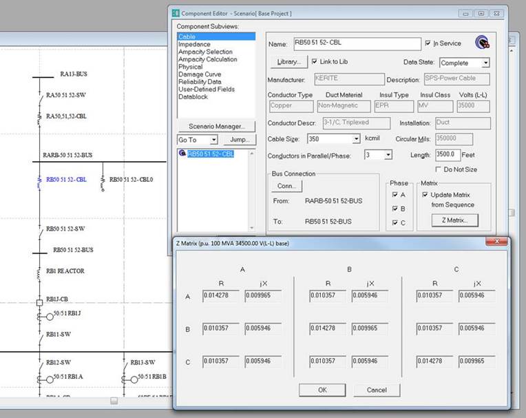
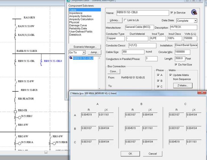
Issues with cables became apparent during the large network tests. While testing the large 2612 node system there was a huge difference in GLD and PTW results. There was an especially large difference in the reactive loads across the lines and this was irreconcilable given the information present in the exports. No amount of change could achieve the results of PTW and worse yet no change could move the GLD calculated Z-matrices toward those calculated by PTW. PTW allows individual checking of Z-matrices which were used for reference of the matrices produced in GLD. Using the same parameters and values as in PTW, and even with some change, there was a large difference which could not be easily accounted for.
Checking the Z-matrices produced with differently branded cables confirmed an idea which had originally sparked the query; large capacitive reactance in the lines. The general cables being used had very high imaginary components, supporting the large difference in capacitance along individual wires which had prompted the investigation. Changing the model to only use a cable type which did not have the large capacitance improved the results only marginally.
No further investigation was done due to an ultimate limiting factor. GLD uses line impedance calculations based on Kersting’s method; a modified version of Carson’s equation. This makes use of a modified Carson equation to calculate the Z-matrix.
The assumptions made by Kersting are fair since systems are driven at 60Hz and with earth resistivity near 100 Ω/m. Assuming ideal conditions for the cables in these modified equations reveals that a minimum impedance value is allowed.
Focusing on the self-impedances shows,
z_ii= r_i+0.09530+j0.12134 {ln(1/GMR_i )+7.93402] Ω/mile
Where r_i=0Ω and GMR_i=1ft,
z_ii=0+ 0.09530+j0.12134 [ln(1/1)+7.93402] Ω/mile,
z_ii=0.09530+j0.12134*[7.93402] Ω/mile,
z_ii=0.09530+j0.96271Ω/mile
is a minimum of a line in GLD.
At 3500ft long, this cable “RB50 51 52-CBL0” shows a minimum resistance of 0.06317 + j0.63816Ω.
| General Cable (Ω) | Kerite Cable (Ω) | Minimum Carson's (Ω) | |
|---|---|---|---|
| Real | 0.05013 | 0.15838 | 0.06317 |
| Reactive | 0.12331 | 0.11054 | 0.63816 |
Comparison table of the self-impedances of the two PTW cables and the minimum allowed by Kersting's method in Ω.
| General Cable (PU) | Kerite Cable (PU) | Minimum Carson's (PU) | |
|---|---|---|---|
| Real | 0.004519 | 0.011161 | 0.005695 |
| Reactive | 0.014278 | 0.009965 | 0.057531 |
Comparison table of the self-impedances of the two PTW cables and the minimum allowed by Kersting's method in PU.
The limiting factor becomes obvious when noticing that all Z-matrix values in GLD are less than the minimum values allowed by Kersting’s method. The reactive impedances are far higher than those which appear in the PTW models. Without the ability to accurately reduce the GLD Z-matrix values to the same range as PTW’s there was no more which could be done. Without changing the method used in GLD itself or calculating the matrices beforehand there is nothing which can be done to achieve better coincidence between PTW and GLD simulation results; at least in large networks.
The proprietary nature of SKMs modeling algorithms, the cables in particular, along with the inability to export Z-matrix data for these cables makes it nearly impossible to verify the effective impedance of GLD cables with those in PTW. Although the same parameters for physical construction are used to define the cables there is no way to ensure that the use of/simulation with said parameters is the same.
Due to the unchanged nature of the ported model it is easy to understand why the coincidence of the large model result is imperfect. Since all basic data is preserved between models only modeling methods of the individual components and the simulation algorithms themselves can cause the discrepancies seen in the results comparisons. This is clear referring back to the 72 node model. Transformers caused some error in the comparison, but cables are also possible contributors based on the 2612 model issues and the voltage error inverse relation to reactive power error. Together the two modeling differences could easily cause the error results seen in both 72 node and 2612 node systems, there being many series cables and transformers from load to utility in each.
Additionally, it should be noted that the PTW model is not used for load flow analysis and has not been verified against neither another software simulation nor the physical network. The component models being used are also not guaranteed to be accurate as seen by the general cables having likely been picked from the built-in library without comparison to the actual network.
Remaining issues pertaining to the exact correspondence of PTW and the ported GridLAB-D results ought to be explored. Due to the efforts made to achieve equivalent models there is no more which can currently be done on this matter. The difference in flow paths and associated error in the GLD model indicates that the cables have a large enough difference in impedance between software that flow paths change completely. The transformers contribute a large part as well due to the number of them in series from load to utility.